ISED 160 NOTES ABOUT HOMEWORK, ANNOUNCEMENTS, ETC.
|
Assigned on: |
BE SURE TO CLICK ON RELOAD/REFRESH ON YOUR COMPUTER OR THE CURRENT ADDITIONS TO THE PAGE MAY NOT APPEAR! You may also not see current pages if your computer does not have an up-to-date browser… download a new version or use a library/lab computer. Scroll down as new assignments are added to the old. New assignments are generally posted by 2:00 pm of the lecture day unless otherwise noted.
|
||||||||||||||||||||||||||||||||||||||||||||||||||||||||||||||||||||||||||||||||||||||||||||||||||||||||||||||||||||||||
|
|
Most current work is listed first, followed by previous
entries: |
||||||||||||||||||||||||||||||||||||||||||||||||||||||||||||||||||||||||||||||||||||||||||||||||||||||||||||||||||||||||
|
Th 12/02 |
We went over the word problems from the last hmk and talked about misleading graphs from section 2.3 in your book. Test 5 on Thursday 12/09 is the last mandatory graded activity for the course. Those who take Test 5 will be finished with the course. Those who miss it will be given an opportunity to replace the missing test with a comprehensive final during finals week. Homework due Tuesday 12/07: Read section 2.3 and then try: 2.3 p96 # 2, 6, 8, 12, 14 TEST 5 FORMAT for Thursday
12/09 : You will be supplied with test and graph paper, formula for slope, forms for equations of lines and exponentials, and equations for the line of best fit (Sxx, Sxy, etc.). You must bring something to write with and a calculator that has log and raising a base to a power keys.
1. Given a problem like 4.2 p206 #21/22, a. Graph the points and draw what you think is the best line thru them, and estimate the line of best fit using point-slope form by picking two points on your line (formulas for slope and equations of lines will be supplied). b. given
the summation table already done ( sums of x, y, xy, x2 , y2) use the equations for the line of best fit to find
the best line to describe the data. I gave you these summations when I
assigned 4.2 #21 to make the work go faster, and I will do the same on the
test! c. use
your line estimate to interpolate (given an x value within known data, plug
into equation to find the y value). This is like part c of 4.2 #21. d. use your line estimate to extrapolate (given an x value outside of known data, plug into equation to find the y value) and see if it looks reasonable. This is like part e of 4.2 #21.
2. Finding the equation of best fit for an exponential: a. graph
given data and estimate an equation for an exponential relationship by
using two points on the curve and y= b(a)x. b.
transform the exponential data into linear data using logs and graph the
result. c. given the line of best fit for the logged data (x, logy), turn the line into the exponential of best fit for the original data by “unlogging” the slope and y-intercept. Then write the equation of the exponential of best fit. 3. Given two
data points, find the line and the exponential thru them and compare extrapolated
values for a given x (like previous hmk problem #1 using points ( 3, 40) and
( 8, 62 )). 4. Given
about two tables of perfectly linear or exponential data (perhaps one of each),
write the linear or exponential equation for each without graphing. Example:
The change in y is +3.2 for
each change of +5 in x, so this is linear with slope 3.2/5=0.64. Then y = 0.64x + 7. If you did not have the y-intercept in the table, you could use y = mx + b and any other point value to solve for it. For instance, if you use (5, 10.2) and m = 0.64 in y = mx + b, you would get: 10.2 = 0.64(5) + b. Solving for b, b = 10.2 – 0.64(5) = 7. Example:
Using the y-intercept for b = 25.000 and the point (4, 84.375) i.e., x = 4 and y = 84.375 with y= b(a)x , 84.375 = (25.000)(a)4. Solving for x, we must divide by 25.000 on both sides, to get (a)4=84.375/25.000 or (a)4=3.375. Now you must raise both sides of the equation to the 1/4 power to solve for a: (a4)1/4=(3.375)1/4 so that a=1.355. So y= 25(1.355)x .
5. Given a
short word problem that describes a linear relationship, write the
appropriate equation and use it to find specified values. Example Suppose that you have $50 left on an out-of-state gift card that you can’t seem to find and the company that issued the card plans to deduct $2 a month from its value as a service fee. Write an equation to describe the situation. a. How much will be left on the card after 10 months? Answer: y= -2x+50 so for x=10, y=30 b. How much will be left on the card after 30 months? Answer: y= -2x+50 so for x=30, y= -10. This is not possible, so you cannot project your model that far into the future. c. When will the card have no value? Answer: y= -2x+50 so for
y=0, x=25 weeks. 6. Given a
short word problem that describes an exponential relationship, write the
appropriate equation and use it to find specified values. Example Suppose that a population of 32,000 is growing exponentially at a rate of 5.7% per year. Write an equation for the exponential relationship. What is the population going to be in 5 years? How long would it take for the city to triple its population by your model? Answer: In 5 years y= 32,000(1.057)5 = 42220.65. To find the time to triple, if y= 32,000(1.057)x and y=96,000, we have 96,000= 32,000(1.057)x which yields 3 = (1.057)x . To solve for x, take the log of both sides of the equation and the log properties give us that x=log 3 / log 1.057 = 19.82 yrs. Example Suppose that in the previous problem the population of 32,000 is decreasing at the rate of 3.5% per year. Write the equation for this exponential relationship and tell how long it would take for the city to have 60% of its original population left. Answer: y= 32,000(1-0.035)x = y= 32,000(0.965)x so when 60% of the original population is left, 0.60= (0.965)x . (That is, 60% of the population of 32,000 is y=0.60*32,000=19,200, so we have 19,200= 32,000(0.965)x which when simplified by dividing by 32,000 yields 0.60. But you do not need to go thru all of that!).To solve for x, we take the log of both sides of the equation and the properties of logs give us that x=log 0.60/ log 0.965 = 14.34 years. 7. One or
two misleading graphs to briefly analyze, like hmk above from 2.3 due on
Tuesday. On Tuesday 12/07, we will go over the hmk, clean up a few ideas, and review items that you have questions about for the test. |
||||||||||||||||||||||||||||||||||||||||||||||||||||||||||||||||||||||||||||||||||||||||||||||||||||||||||||||||||||||||
|
T 11/30 |
Practice linear and exponential word problems: 1. Suppose that a car rental company charges a flat fee of $15 plus a per mile fee of 12 cents. a. What will be owed to the company for the rental if the customer drives 245 miles? Answer: y=0.12x+15 so for x=245, y=44.40 b. For what number of miles will the rental bill total come to $70? Answer: y=0.12x+15 so for y=70, x=458.3
2. Given the following exponential functions, state the initial amount present and the rate of growth or decay (indicate which!) as a percentage. a. P(t) = 678 (1.072)t b. P(t) = 2.07 (0.723)t Answer: In part a, the initial value is 678 (the y intercept) and it is growing at the rate of 7.2% since 1.072 = 1 + 0.072. The rate of increase in an exponential is the amount that the factor a in the exponential is above 1 (or 100%). So in this case, the rate of increase is 0.072 = 7.2%. In part b, the initial value is 2.07 and it is decaying at the rate of 27.7% since the rate of change for a decreasing exponential is the amount that the factor a in the exponential is below 1 (or 100%). So in this case, since 0.723=1– 0.277, the rate of increase is 0.277 = 27.7%.
3. Suppose that for a certain type of bacteria, we start with a population of 1000 and we know that this type grows exponentially at a 49% rate. Write the exponential equation for the number of bacteria present as a function of time in hours. How many bacteria are present after 2 hours? How many after 5 hours? Answer: y= 1000(1.49)x which when x=2, y=2220 and when x=5, y=7344.
4. Suppose that a population of 50,000 is growing exponentially at a rate of 4.5% per year. Write an equation for the exponential relationship. a. How many will be in the population after 10 years? Answer: y= 50,000(1 + 0.045)x = 50,000(1.045)x . When x=10, y=77,648.47, or about 77,648. b. How long would it take for the city to double its population by your model? Answer: y= 50,000(1.045)x so when y=100,000, we have 100,000= 50,000(1.045)x which when simplified by dividing by 50,000 yields 2= (1.045)x . To solve for x, we take the log of both sides of the equation and the properties of logs give us that x=log 2 / log 1.045 = 15.7 yrs.
5. Suppose that in the previous problem the population of 50,000 is decreasing at the rate of 10% per year. Write the equation for this exponential relationship and tell how long it would take for the city to have 75% of its original population left. Answer: y= 50,000(1-0.10)x = y= 50,000(0.90)x so 75% of the population of 50,000 is y=0.75*50,000=37,500, so we have 37,500= 50,000(0.90)x which when simplified by dividing by 50,000 yields 0.75= (0.90)x . To solve for x, we take the log of both sides of the equation and the properties of logs give us that x=log 0.75 / log 0.90 = 2.73 years.
Homework due Thursday 12/02: 1. Given the data points (
3, 40) and ( 8, 62 ): a. Find the equation of the
line thru the points (use point-slope form to solve for m and b) b. Find the equation of the
exponential thru the points (use y= b(a)x and solve for a and b). c. If the y coordinate
stands for a city’s necessary operating budget in millions of dollars (i.e.,
if y = 5, then the budget is $5,000,000) and x stands for years since 2000,
and the city manager mistakenly projects the future operating budget from
this data as growing linearly when it is actually growing exponentially, how
many millions of dollars shortfall will the city experience in 2015? 2. During the period after
birth, a male rat gains exactly 40 grams per week. Assuming that the rat
grows at a steady rate, and that he weighed 100 grams at birth, give an
equation for his weight after x weeks. (1 pound = 453.59237 grams) a. What is the rat’s weight in both grams and pounds according to your model after 5 weeks? b. When would the rat weigh 500 grams? c. Would you be willing to
use this line to predict (extrapolate) the rat's weight at age 2 years? (Give
answer in terms of both grams and pounds). 3. A town has a population of 12,300 people and the population is decreasing exponentially at the rate of 15.5% per year. a. How many people will be in the town in 2 years if this trend continues? b. When will the town have
half of its original population? 4. Suppose in problem #3,
the population is increasing exponentially at the rate of 15.5% per year. a.
When will the town’s population double? b. When will the town’s
population be 2.5 times its starting population of 12,300? |
||||||||||||||||||||||||||||||||||||||||||||||||||||||||||||||||||||||||||||||||||||||||||||||||||||||||||||||||||||||||
|
Th 11/18 |
We do not meet next
week…have a great Thanksgiving! Supplemental notes to our work in class today
follow (exponentials not in our version of the book), with hmk below due
after the break! Finding the exponential of best fit for a
scatterplot of exponential data by using logarithms to turn it into a linear
scatterplot.
If you have a scatterplot of linear data, you saw in class last time that it was relatively easy and accurate to estimate the line of best fit from a graph and also find the best fit line using the equations from last time. However, if you have a scatterplot of data that is best described by an exponential curve, it is difficult to draw a good curve and you wouldn’t know how to find its equation because it does not have a constant slope (i.e, you could not take two points and use the slope formula or point-slope form!).
But if you take the same x values but the logarithm of each y value in the exponential data, that is, turn (x, y) into (x, logy) in the table, you will have transformed it into linear data! From here, you could come up with a good linear estimate or use the equations for line of best fit to find y = mx+b for the “logged” data (x, logy). Then you can “unlog” the slope m and y-intercept b to find the “a” and “b” in y= b(a)x for the original data.
We did an example of this process in class. Here is another example, but with data that is not perfectly exponential as it was in class: The following below set of data is best represented with an exponential relationship y= b(a)x but since it is not perfectly exponential, we cannot write the relationship from the table values.
It is difficult to estimate an exponential scatterplot relationship, but it can be turned into a linear relationship by taking the logarithm of the y values (graph it if you don’t believe it!).
Now we can find the best fit line for this (x, logy) linear scatterplot by making a summations table with and use the standard deviation calculations (Sxx, etc.) for finding the best fit line.
Sxx = 26-(64/3)=4.67 Sxy = 18.26-[(8)(7.09)/3]= -0.65 slope = -0.65/4.67 = -0.14 y-intercept = 2.36-(-0.14)( 2.67) =2.73 So the best fit line for the logged data is y=-0.14x+2.73
To find the best fit exponential for the original data, “unlog” the slope and y-intercept of the line above: raise 10 to the power of each separately and then write the equation for the exponential of best fit for the original table data (x, y). a=10slope =10-0.14 = 0.72 b=10y-intercept = 102.73= 537.03 So the best fit exponential for the original data is y=537.03(0.72)x.
(Check your answer: does plugging x=1 into your best fit exponential give you something close to the original table value of 398.11? It shouldn’t be exact because the original data was not perfectly exponential, but it should be in the ballpark! Same for the other two points.). Notice that this is a decreasing
exponential relationship. For decreasing exponential relationships, a<1
and for increasing exponential relationships, a>1. For decreasing linear
relationships y=mx+b, m is negative and for increasing ones, m is positive.
We will talk more about this next week. How to estimate
the equation of best fit for an exponential (only good enough for a rough
estimate, since small errors are magnified greatly by exponentiation):
Example Estimate the exponential equation that passes thru (0, 28) and (5, 86) in the form y= b(a)x . Your estimate for b is 28 from the point (0, 28), and now you have to find a. Take the other point (5,
86) and plug in the x and y values in y= b(a)x : Since x = 5 and y = 86, y=
b(a)x
becomes 86= 28(a)5 which gives 86/28 = (a)5. To find a, you must raise
86/28 to the 1/5th power. That is, (86/28)1/5=(3.07)0.20=1.25. Now we have the equation y=
28(1.25)x . This is an increasing exponential since a > 1. Example Estimate the exponential equation that passes thru (0, 200) and (3, 24) in the form y= b(a)x . Your estimate for b is 200 from the point (0, 200), and now you have to find a. Take the other point (3,
24) and plug in the x and y values in y= b(a)x . Since x = 3 and y = 24, y=
b(a)x becomes 24= 200(a)3 which gives 24/200 = (a)3. To find a, you must raise 24/200 to the 1/3rd power. That is, (24/200)1/3=(0.12)1/3=0.49. Now we have the equation y=
200(0.49)x . This is a decreasing exponential since a < 1. Example Estimate the exponential equation that passes thru (3, 5) and (7, 15) in the form y= b(a)x . Now you have to find an estimate for both a and b. Take the point (8, 15) and
plug in the x and y values in y= b(a)x to get 15= b(a)7. Take the point (3, 5) and
plug in the x and y values in y= b(a)x to get 5= b(a)3. Divide the first equation
by the second equation: To find a, you must raise 3 to the 1/4th power. That is, (3)1/4 = 1.32. Now we have the equation y= b(1.32)x . We still need to find b, and can do this using either point: Take the point (3, 5) and
plug in the a, x, and y values in y= b(a)x to get 5 = b(1.32)3. Solve for b: b = 5/(1.32)3 = 5/2.30 = 2.17. Now we have the equation y
= 2.17(1.32)x .
Homework (due Tuesday 11/30): The first two problems are linear, as with your last hmk. For these, I am giving you the table summations to cut down on your work. Use the Sxx, Sxy equations using them, though, to find the best fit line equation first. You do not have to graph this data if you don’t want to. The third problem involves logarithms and is done in the same way as the extra example in the first half of today’s notes above.
1. Do 4.2
p206 #21 parts a (line of best
fit), c (skip the “residual”), e (not good to project too far!) given that 2. Do 4.2
p207 #22 parts a (line of best
fit), c (skip the “residual”), e (not good to project too far!) given that
3. The following table is of an exponential scatterplot (not perfectly exponential, but is best described by an exponential function). Do as in the example in the notes above:
a. Take the original (x, y) values in the table and make a new table (x, log y). That is, find log 25, log 34.12, etc., to start with…
b. Using
the values in the (x, logy) table, find the line of best fit using Sxx and
Sxy. Hint: you should get the following summations to plug in (find and check them for yourself):
(For y notice that you are not summing the original y values to get 619.35— you sum the logged y values to get the y summation of 9.66!):
c. Convert the slope m and the y intercept b from the best fit line for the (x, logy) data in part b to the “a and b” that are the components of the best fit exponential y= b(a)x for the original (x, y) data. This is done by a=10slope and b=10y-intercept . (This is “unlogging” the data). Does this equation look like it describes the data well? Compare with a graph of the original data.
d. Use your estimate for the best fit exponential from part c to estimate the value of y when x is 3.8. e. Graph the data points in the original table (informal graph on binder paper) and draw what you think is a good best exponential curve through them. Estimate the y coordinates of the points from your graph for x = 1 and x = 3. Use these points to estimate the equation of the exponential curve you drew, using the method in the second half of the notes above (How to estimate the equation of best fit for an exponential). Does it match part c well?(it probably will not). |
||||||||||||||||||||||||||||||||||||||||||||||||||||||||||||||||||||||||||||||||||||||||||||||||||||||||||||||||||||||||
|
T 11/16 |
Today we worked on linear scatterplots, and Thursday we will work on exponential scatterplots. The exponential part is in the more expensive version of this text, but I did not think it was worth the price to buy that version just for that one missing topic, so I will supplement your version with notes here about exponentials. That means it is very important for you to be in class and read the notes here for the next few sessions!
Reading in the text: --Read 4.1 p177-179 objective 1 “Draw and interpret scatter diagrams” --Read 4.2 p195-200 example 1 and objective 1 “find the least squares regression line…” and note that I am using the equations at the bottom left of p198 (the “equivalent form” for slope is Sxy/Sxx) because the computation of “r” in the blue box is more complicated and involves more computations than the equivalent form. Look at the table on p182 example 2, where they compute r using the “deviations” for x and y from their respective means. The other way, which we did in class, is easier!
Supplementary notes on lines of best fit (equivalent form from p198): Given several data points
(x,y) you fill out the table below (the data points' coordinates are the x
and y values. The symbol For example, for the data points (2,7) and (4,8) we know that the slope of the line thru them is 1/2 = 0.5 so that y-7 = 0.5(x-2) so that y = 0.5x +6 is the equation of the line thru them, that is, a line with slope 0.5 and y-intercept 6. Now let us use the equations for the line of best fit: Set up a table with the following quantities and sum them up
(n=2 in this short ex. for the 2 data pts given)
After having done this with all of the given data points use all of these numbers to plug into the formulas for the line of best fit (which are below) Sxx = Sxy = Slope of best line = Sxy/ Sxx = 1/2 = 0.5 Y-Intercept of best line = The best fit line is then y=0.5x+6 (which matches the equation found at the beginning exactly, because 2 points make a line, not a scatterplot!
Another example: For the data pts (1,9), (2,8), (3,6), and (4,3):
Note that n=4 is the number of data points
Using the formulas above, Sxx = 30-(100/4)=30-25=5 Sxy = 55-[(10)(26)/4]=55-65= -10 Slope = -10/5= -2 Y- intercept = 6.5-(-2)(2.5) =6.5+5 =11.5 The best fit line is then y= -2x+11.5
Supplementary notes on linear and exponential patterns (not in book): Before the end of class, we spent a few minutes talking about the differences and similarities of linear and exponential (one kind of non-linear) functions. Given a table of perfectly linear or exponential data, we can write the appropriate equation that describes that data in the form y=mx+b for a line or y= b(a)x for an exponential. The b in both cases is the y-intercept and is found in the table where x=0. With linear relationships, m is the slope of the line and is the amount by which we add each time. We add positive numbers for an increasing line (positive slope) or negative numbers for a decreasing line (negative slope). For instance, if the slope is 5, then mx = 5x = x+x+x+x+x. After the sum mx is found, b is also added on to get y=mx+b. So a linear relationship is one built by repeated addition. The a in the exponential is the amount by which we multiply each time (“a” contains the rate of increase or decrease since a=1+r or 1-r, where r is the rate—we will talk more of this next time). In y= b(a)x , the (a)x means “a” multiplied by itself x times. For instance, (2)5 = 2*2*2*2*2 = 32. After you find (a)x and then multiply by the b to get y= b(a)x you can see that an exponential relationship is built by completely by multiplication.
The following are some tables of data to illustrate what sets of linear and exponential data look like and how their equations are written:
is a decreasing linear set of data because you are adding -3 each time, so y=-3x+12. (Verify that the points in the table lie on this line by plugging the values in and checking them).
is a increasing linear set of data because you are adding +7 each time, so y=7x+20.
is an increasing exponential set of data because you are multiplying by 3 each time so y= 12(3)x. (plug the x and y values into the exponential equation above and see that it gives a true statement). Note the placement of the y-intercepts of each above and how 3 and 12 are used in each!
is a increasing exponential set of data because you are multiplying by 1.5 each time so y= 50(1.5)x.
is a decreasing exponential set of data because you are multiplying by 0.9 each time so y= 250(0.9)x.
is a decreasing exponential set of data because you are multiplying by 0.75 each time so y= 420(0.75)x.
HOMEWORK due Thursday 11/18: 1. Look at the data set in 4.2 p204 #9. a. Graph the data informally, draw what you think is the line of best fit, and estimate your line’s equation using two points on your line that are not original data points. b. Make a table of x, y, xy, xsquared values and use the equations Sxx, Sxy, etc. above to find the actual line of best fit. c. Using their method, they get y = -0.7136x + 6.55. Do you get the same?
2. Look at the data set in 4.2 p204 #10. a. Graph the data informally, draw what you think is the line of best fit, and estimate your line’s equation using two points on your line that are not original data points. b. Make a table of x, y, xy, xsquared values and use the equations Sxx, Sxy, etc. above to find the actual line of best fit. c. Using their method, they get y = 0.1457x + 1.1370. Do you get the same?
3. Given the tables of values for functions, decide if the data are best represented by a linear function or an exponential function (do the values change by addition or multiplication?). Write the equation for the relationship that you decide for each table.
|
||||||||||||||||||||||||||||||||||||||||||||||||||||||||||||||||||||||||||||||||||||||||||||||||||||||||||||||||||||||||
|
T 11/09 |
Test 4 was completed today. I will post the test 4 grades by Thursday afternoon at: http://www.smccd.edu/accounts/callahanp/test160F10.html (your first three test scores are there now—if you need
your code, email me). Thursday 11/11 is Veteran’s Day, so no classes meet on campus
that day. Tuesday 11/16 is the last day I will sign withdrawals. If after seeing your test #4 grade you decide to withdraw, you must turn in the completely filled out paperwork to the DAIS office BH 239 before 11/16 so that I will be sure to get it.
Before the test, I talked about some material about graphing from Algebra, that you should review so that we can start our last segment on visual representations of data (you do not need to get graph paper).
Start by reading 4.2 p196/197 example 1 in your book. It reviews finding of slopes and writing the equation of a line. Read ahead in that same section to see what we will work on in class on Tuesday (scatter plots and linear regression).
GRAPHING practice for next week! You must know how to find the slope of a line from the coordinates of two points on the line, where you are also able to estimate the coordinates of those points from a graph. The slope of a line measures the change in y values over the change in x values:
Slope m =(y2 - y1 )/(x2 - x1 )
You must know how to use point-slope form for the equation of a line: y - y1 = m ( x - x1 )
And how to put a line into slope-intercept form:
y = mx + b
For example:
Suppose the points ( 2.3 , 12.7 ) and ( 3.4 , 22 ) lie on a line. Slope m =(y2 - y1 )/(x2 - x1 )=(22-12.7)/(3.4-2.3)=9.3/1.1=8.45
We can use either of the
two points above to be (x1,y1) in point-slope form and
solve for y: y - 12.7 = 8.45 ( x - 2.3 ) y - 12.7 = 8.45(x) + 8.45(- 2.3 ) y = 8.45x - 19.44 +12.7 y = 8.45x - 6.74
To use this equation to make predictions, suppose that x stands for time in years and y stands for profit in millions of dollars for a company. Using the equation above, how much profit will the company realize in 5 years? This means that we plug in 5 for x and find y = 8.45(5) - 6.74 = 42.25 – 6.74 = 35.51, that is, 35.51 million dollars in profit is projected.
You might want to visit the
interactive web links below if you want more practice. The coolmath site is
geared toward kids, but at least it gets to the point of the problems
quickly. Otherwise, search for another site or an old Algebra book can be
consulted! http://www.coolmath.com/algebra/08-lines/06-finding-slope-line-given-two-points-01.htm http://www.coolmath.com/algebra/08-lines/11-finding-equation-line-point-slope-01.htm http://www.coolmath.com/algebra/08-lines/12-finding-equation-two-points-01.htm
Work on being proficient in the above tasks so that we can more easily work on an activity in class on Tuesday. Be careful about missing class the last few weeks, as things will go quickly towards the end, and Test #5 is a mandatory part of your grade and cannot be dropped!
Homework (due Tuesday 11/16): 1. Find the slope of the line that passes thru the points ( 2.5 , 256.5 ) and ( 10.7 , 42.8 ). Round calculations to 2 decimal places. 2. Write the equation of the line above using point-slope form with the point ( 2.5 , 256.5 ) and solve for y to put it in slope-intercept form. 3. Write the equation of the line above using point-slope form with the point ( 10.7, 42.8) and solve for y to put it in slope-intercept form. (Notice that your answers should be close for parts 2 and 3, but rounding may cause a small difference). 4. Graph
the points from part 1 on an informal graph with equal marks of size 1 on the
x axis from 1 to 10 and equal marks of size 50 on the y axis (0, 50, 100,
150, 200, 250), and draw a straight line through them. Extend the line to the
y axis. Does the y value where the line crosses the y axis match the number b
from slope-intercept form y= mx + b that you found in parts 2 and 3? It
should be close, but don’t expect too much from an informal graph! 5. Use your line’s equation from part 2 or 3 to predict y when x is 20. |
||||||||||||||||||||||||||||||||||||||||||||||||||||||||||||||||||||||||||||||||||||||||||||||||||||||||||||||||||||||||
|
Th 11/4 |
I issued 3-digit personal
codes at the end of class today, so that you could check the “testscores”
link on this website’s index page to check what I have for you so far for
tests 1, 2, and 3. I uploaded them by 5pm, so if you don’t see them, you may
need to refresh/reload the page. If you were not there to receive your code,
you can email me for the code or just get it on Tuesday. Test 4 will occur as scheduled on Tuesday 11/09 Not much to calculate on this test. The form that I have put the examples below in is the form I want you to use on the test. The following examples are not meant to cover every problem type, they are there just to help guide you in the format of the test. You are responsible for all types of problems that we did in class and for homework.
1. One problem to compute a given nCr showing the meaning of factorial and how to cancel part of the numerator with the denominator and finding the value. For example, 50C3=(50!)/(3!)(47!)=(50*49*48*47****2*1)/(3*2*1)(47*****2*1) so the (47*****2*1) in top and bottom cancel to leave (50*49*48)/(3*2*1)=19600
2. About 4 or 5 situations where you must decide if order matters or not and indicate the appropriate nPr or nCr notation without actually computing it (however, you must include what numbers are used for n and r). For example: In how many different ways can Bob pick a best man and a verse reader from his 5 closest friends for his upcoming wedding? Answer: 5P2
3. About 5 or 6 probabilities where you form a quotient of nCr values in the classical probability sense where you can use + and * without worrying about whether sets or disjoint or events are independent (where you do not have to use the general addition or multiplication rules). You must know the subsets of a deck of cards and how to perform other probability problems done for hmk. For example: a. P(2 hearts in 2 drawn )=13C2/52C2 b. P(a heart or a club) in 1 card drawn= (13C1+13C1)/52C1 c. If a bag of 100 tulips has 40 red, 35 yellow, and 25 purple tulips, one selected at random, then P(red)=40/100 d. Same bag as in part f, two selected, P(red or purple)= (40C1+25C1)/100C2 e. If a set of 30 dishes has 4 broken, what is the probability that in six dishes selected at random, one is broken? (4C1*26C5)/30C6 f. If a certain lottery asks you to pick 4 regular numbers from 52 and 1 Mega number from 17, what is the probability of getting 1 of the winning regular numbers and not getting the Mega number? (4C1*48C3)/52C4 multiplied by 16C1/17C1 (Below, I have split
the “type 4” test problems from the review in class into two separate
problems #4 and #5 for easier reading, and renumbered “type 5” test problem
as #6) 4. Problems where you show knowledge of the general addition rule (provided). These involve problems where the sets in question share items at the same time, that is, not disjoint and have an intersection. For example, in one card drawn, P(a face card or a red card)=12/52+26/52-6/52= 32/52 5. Problems where you demonstrate the multiplication rule (provided). For example, a. If 19.1% (0.191) of homes are in the Northeast and 4.4% (0.044) of homes earn $75,000 per year or more and are located in the Northeast, what is the probability that a randomly selected home earns more than %75,000 per year, given that the home is in the Northeast? You are trying to find P( >75,000 given Northeast) so let it be x in the equation formed using the general multiplication rule and solve for x: P(>75,000 and Northeast) = P( >75,000) * P( >75,000 given Northeast), i.e., 0.044 = 0.191*x x = 0.044/0.191 = 0.23 b. If a bag of 100 tulips has 40 red, 35 yellow, and 25 purple tulips, two selected at random, P(1st red and 2nd purple)=P(1st red)*P(2nd purple given 1st red)=(40/100)*(25/99)
6. A table from which to write probabilities and demonstrate the general addition and multiplication rules, as in hmk 5.2 p248 #39, 40 and hmk 5.4 p262 #17,18 For example, if one person from the survey is selected at random:
a. P(male and married) = P(male)*P(married given male) = (95.0/197.4)*(58.6/95.00) = 58.6/197.4 b. P(male or married) = P(male) + P(married) – P(male and married) = (95.0/197.4) + (117.9/197.4) – (58.6/197.4) = 154.3/197.4 |
||||||||||||||||||||||||||||||||||||||||||||||||||||||||||||||||||||||||||||||||||||||||||||||||||||||||||||||||||||||||
|
T 11/2 |
Reading assignment: The general addition rule
is in 5.2 p241-243 (including up thru example 4) and has to do with the union
of two sets and says that the probability that either event A or event B
occurs is: P(A or B)=P(A)+P(B)-P(A and B) The general multiplication rule is in 5.4 p255-260 (but skip example 5 p259) and has to do with the intersection of two sets and says that the probability that both A and B occur is: P(A and B)=P(A)*P(B given A), where P(A) is used to mean “the probability that event A will occur”, P(A and B) means “the probability that both events A and B will occur”, and P(B given A) is what is called a conditional probability, and means “the probability that B occurs, given that we know A has occurred already” or “the probability that B occurs, given that we know we are making selections only from A”. The book uses a “slash” for “given that”, but I find that writing out “given” makes it more clear. Using the general multiplication rule to find card probabilities can become very involved. That is why I like to focus on the concept of conditional probability through the use of tables, where it is much easier to see some validation for why the general multiplication rule works. However, there are some book problems that ask you to interpret a word problem situation in terms of the general rule. So I include some examples:
Examples from the book:
5.2 p247 #29c P(ace or heart) = P(ace) +P(heart) – P(ace and heart) = 4/52 + 13/52 – 1/52 = 16/52
5.2 p248 #39 a. P(satisfied) = 231/375 b. P(junior) = 94/375 c. P(satisfied and junior) = 64/375 from the intersection of the row and column in the table, or by the general multiplication rule from 5.4, P(satisfied and junior) = P(satisfied) * P(junior given satisfied) = 231/375 * 64/231 = 64/375 Note that (junior given satisfied) means that you are selecting only from those who were satisfied, and that is out of a total of 231, not 375! d. P(satisfied or junior) = P(satisfied) + P(junior) – P(satisfied and junior) = 231/375 + 94/375 – 64/375 = 261/375
5.4 p262 #11 P(spade) = 13/52 P(black and spade) = P(black) * P(spade given black) Or 13/52 = 26/52 * P(spade given black) So solving by multiplying both sides by the reciprocal of 26/52 (which is 52/26), P(spade given black) = 13/52 * 52/26 = 13/26
5.4 p262 #13 P(cloudy and rainy) = P(cloudy) * P(rainy given cloudy) Or 0.21 = 0.37 * P(rainy given cloudy) So solving by dividing both sides by 0.37, P(rainy given cloudy)= 0.21 / 0.37 = 0.57
5.4 p262 #17 To use this table to find probabilities, you must find the totals for each row and column. For this problem, we only need the total for “<18” = 49473+19662+8531 = 77666 and the total for “none” = 8531+25678+9106+258 = 43573 a. P(none given <18) = 8531/7666 = 0.11 b. P(<18 given none) = 8531/43573 = 0.20
5.4 p263 #27 Using the general
multiplication rule, a. P(1st red and 2nd red) = P(1st red) * P(2nd red given 1st red) = 12/30 * 11/29 = 132/870 = 0.15 b. P(1st red and 2nd yellow) = P(1st red) * P(2nd yellow given 1st red) = 12/30 * 10/29 = 120/870 = 0.14 c. P(1st yellow and 2nd red) = P(1st yellow) * P(2nd red given 1st yellow) = 10/30 * 12/29 = 120/870 = 0.14 d. no order is mentioned, so you can use the nCr count method: P(red and yellow) = (12C1 * 10C1) divided by 30 C2 = (12*10)/435 = 0.28 Or, add parts b and c to get the same thing: P(red and yellow) = P(1st red and 2nd yellow) or P(1st yellow and 2nd red) = 0.14 + 0.14 = 0.28
HOMEWORK due Thursday 11/04: (very similar to the examples above!) 5.2 # 30c, #40 5.4 #12, 14, 18, 28 |
||||||||||||||||||||||||||||||||||||||||||||||||||||||||||||||||||||||||||||||||||||||||||||||||||||||||||||||||||||||||
|
Th 10/28 |
Today, we took the counting method from the last homework problem one step further with a great real-life probability application: the Lottery. The “nCr” counting method from 5.5 forms sophisticated counts and verifies probabilities listed on the back of a California Lottery playslip.
THE CALIFORNIA LOTTERY: SUPER LOTTO PLUS (homework follows these notes!) To play, you are asked to pick 5 different numbers from 1 to 47 and one “Mega” number from 1 to 27. The top prize (advertised in millions) goes to whoever matches all 5 of 5 winning numbers and the one Mega number. Much smaller prizes are awarded for matching some of the numbers. Prizes are awarded to the following winning combinations:
* Approximate prize info
from source other than the California Lottery: actual prizes may vary! It is helpful to map out the strategy for outcomes by breaking down each number set into the important subsets and see how many are to be taken from each. The last probability below (just before the homework set) “getting any 3 of 5 and not getting the Mega” would be written:
Which translates to : (* means multiply) ((5C3*42C2)/47C5) * ((1C0*26C1)/27C1) In summary, here are the first six outcomes: Getting all 5 of 5 and the Mega: ((5C5*42C0)/47C5) *
((1C1*26C0)/27C1) = (1/1,533,939) * (1/27) = 1 / 41,416,353 = 0.000000002 as above.
Getting all 5 of 5 and not getting the Mega: ((5C5*42C0)/47C5) *
((1C0*26C1)/27C1) = (1/1,533,939) * (26/27) = 26 / 41,416,353 = 0.000000628 = 1/1,592,937 as above.
Getting any 4 of 5 and the Mega: ((5C4*42C1)/47C5) *
((1C1*26C0)/27C1) = ((5*42)/1,533,939) * (1/27) = 210 / 41,416,353 =0.000005070 = 1/197,221 as above.
Getting any 4 of 5 and not getting the Mega: ((5C4*42C1)/47C5) *
((1C0*26C1)/27C1) = ((5*42)/1,533,939) * (26/27) = 5460 / 41,416,353 = 0.000131832 = 1/7585.41 rounded to 1/7585 above.
Getting any 3 of 5 and the Mega: ((5C3*42C2)/47C5) *
((1C1*26C0)/27C1) = ((10*861)/1,533,939) * (1/27) = 8610 / 41,416,353 = 0.00207889 = 1/4810.26 rounded to 1/4810 above.
Getting any 3 of 5 and not getting the Mega: ((5C3*42C2)/47C5) *
((1C0*26C1)/27C1) = ((10*861)/1,533,939) * (26/27) = 223860 / 41,416,353 = 0.005405111 = 1/185.01 rounded to 1/185 above.
Homework Problems for you to do (due Tuesday):
A. Compute the following 6 probabilities (refer to the 6 examples I did above for guidance):
Getting any 2 of 5 and getting the Mega, Getting any 2 of 5 and not getting the Mega, Getting any 1 of 5 and getting the Mega, Getting any 1 of 5 and not getting the Mega (done in class), Getting none of the 5 and only getting the Mega, and Getting none of the 5 and not getting the Mega.
To make your life a little easier, here are some answers to the combinations you will use so that you do not have to find them using factorials and cancellations: nC0=1 for all n, for example, 5C0 = 1 nC1=n for all n, for example, 5C1 = 5 nCn=1 for all n, for example, 5C5 = 1 5C2=10 42C3=11,480 42C4=111,930 42C5=850,668 47C5=1,533,939
B. Try to explain why 3 of the 6 you computed above are excluded from the prize categories at the top of this exercise.
C. The old California Lottery did not have the Mega number. You had to pick 6 winning numbers choosing from numbers 1 to 49. Compute the odds of winning that game. Why do you think they changed the game? |
||||||||||||||||||||||||||||||||||||||||||||||||||||||||||||||||||||||||||||||||||||||||||||||||||||||||||||||||||||||||
|
T 10/26 |
The quiz today
was: If one card is
drawn from a deck of cards, what is the probability that it will be red or
black? Answer: P(red
or black)= (26C1 + 26C1) / 52C1 = (26+26)/52 = 52/52 = 1 = 100%. This was an
application of the “addition rule” (that if you see two probabilities
connected by “or”, you add them). If you draw one card, there is a 100%
chance that it will be either red or black, because those are the only colors
available in the deck! This example was given to convince you that the
addition rule works. For more examples, read the supplementary notes below
(especially if you missed class today). Reading from the book: (taking some basic concepts from each of the sections before we look at more complicated ones) 5.1 section 3 “compute and interpret probabilities using the classical method” p227-230 5.2 see bottom blue box p238 “addition rule for disjoint events” , then read example 2 p240 5.3 see blue box p251 “multiplication rule for independent events”, then read examples 2 and 3 p251/2 5.5 examples 14 and 15 (read this one carefully!) p275 The probability that an event occurs can be formed by using the classical method, that is, by forming the following quotient (fraction): (the # of ways to get a “success”) / (the total # of equally likely things that could occur).
We will form the top and the bottom of the above fraction with nCr counts to start with, because in the probabilities we will focus on for now, order does not matter. With cards, the order in which you shuffle them in your hand does not change the set of cards you have. Permutations come into play with more difficult probability situations that we probably will not have time for.
Note that in general, nC1 = n. For example, 52C1 = 52. But there is no shortcut for 52C2: 52C2= 52!/(2!)(50!)= (52x51x50x49x….x2x1)/(2x1)(50x49x8x…x2x1)=1326. This represents how many pairs can be taken from a deck of cards, where order doesn’t matter. So it is not so easy to just count cards as the problems get harder and involve taking more cards at a time!
Supplementary card examples: The following are some more “simple” examples of writing probabilities using the nCr notation from section 5.5 (not simple as in easy, but meaning not involving compound events where more than one thing is happening!). Count the cards involved in each event and you will see where most of the numbers are coming from (there are 4 aces, 26 red cards, 13 hearts, etc.):
Probability of an ace in 1 draw =4C1/52C1=4/52=0.08 Probability of a red card in 1 draw =26C1/52C1=26/52=0.50 Probability of a diamond in 1 draw =13C1/52C1=13/52=0.25 Probability of a face card in 1 draw =12C1/52C1=12/52=0.23 Probability of a black four in 1 draw =2C1/52C1=2/52=0.04 Probability of a red face card in 1 draw =6C1/52C1=6/52=0.12 Probability of a non-face card in 1 draw =40C1/52C1=40/52=0.77 Probability of 2 aces in 2 drawn =4C2/52C2=6/1326=0.005 Probability of 2 hearts in 2 drawn =13C2/52C2=78/1326=0.06 Probability of 2 face cards in 2 drawn =12C2/52C2=66/1326=0.05 Probability of 3 Kings in 3 cards drawn =4C3/52C3=4/22100=0.0002
The following “compound” probabilities are more difficult than the “simple” ones above, since there is more than one event involved. This involves more difficult questions involving intersections (multiplication rule) and unions (addition rule) of sets. We will talk about these rules more formally later, but for now, we can apply the rules to less complex problems in the following way: When you see the key word “and” in a sentence, from p251 use multiplication to connect the two counts together. When you see the key word “or” in a sentence, from p238 use addition to connect the two counts together:
1. What is the probability of getting a 3 and a 4 in two cards drawn? Answer: (4C1*4C1)/52C2=(4C1*4C1)/52C2=(4*4)/1326=0.01 2. What is the probability of a jack and an ace in 2 drawn Answer: same as the previous one, since they are both still “kinds” of cards! 3. What is the probability of a jack or an ace in 1 card drawn Answer: (4C1+4C1)/52C1=(4+4)/52=0.15 4. What is the probability of getting a diamond and a heart in two cards drawn? Answer: (13C1*13C1)/52C2=(13*13)/1326 =0.13 5. What is the probability of a heart or a club in 1 card drawn Answer: (4C1+4C1)/52C1=(4+4)/52=0.15
Non-card examples that take the multiplication rule farther: (using the above notation, but it is more difficult—it is not just about card counting, but using the basic addition and multiplication principles in making real-world counts!)
For 5 identical job positions there are 12 applicants, 8 of whom are female. What is the probability that in filling these 5 positions, we will get 3 females? This is using the techniques from card counting above in the same way, but with a different set and subsets: Answer: Out of 12 applicants we will take 3 of 8 females AND (multiply) 2 of 4 males, for a total of 5 people hired out of 12 who applied.
(8C3*4C2)/12C5=(56*6)/792 =0.42
Another example: If a set of 30 dishes has 4 broken, what is the probability that in six dishes selected at random, one is broken?
(There are some IMPLIED facts that must be taken into account. If 4 are broken, 26 are not broken and if we take 6 dishes total where 1 is broken, it must mean that we are taking 5 that are not broken) so (4C1*26C5)/30C6
Examples from the book (mostly non-card examples): 5.1 p234 (using the set-up for probabilities on p227) 29. P(sports) = 288/500 = 0.576 31. a. P(red) = 40/100 = 0.40 b. P(purple) = 25/100 = 0.25 33. b. P(8) = 1/38 = about 0.03 c. P(odd) = 18/38 = about 0.45 47. a. P(right) = 24/73 = about 0.33 b. P(left) = 2/73 = about 0.03 5.2 p247 (use the nCr notation as in the card examples above with the addition rule) 29. a. P(heart or club) = (13C1 + 13C1)/52C1 = (13+13)/52 = 26/52 = 0.50 b. P(heart or club or diamond) = (13C1 + 13C1+13C1)/52C1 = (13+13+13)/52 = 39/52 = 0.75 5.5 p277 62. c. (55C3*45C4)/100C7 = (26235*148995)/(1.60075608x10 to the 10th power) = about 0.24 65. a. Out of the 13 tracks, 5 are liked so 8 must be disliked. You are taking 2 of 5 liked and 2 of 8 disliked for the event probability on the top of the fraction. On the bottom of the fraction, any 4 could pop up from the 13 tracks available.
(5C2*8C2)/13C4 = (10*28)/715 = about 0.39
HOMEWORK: (will be collected on Thursday—I am looking for effort, not necessarily all the right answers, so read your book and the notes above and give the following your best try!): Card problems (use the card examples above for
reference): 1. State the probability
using the classical method as a fraction in nCr notation: In 1 card drawn from a deck, what is the probability that it will be a heart? 2. State the probability
using the classical method as a fraction in nCr notation: In 2 cards drawn from a
deck, what is the probability that they will both be fives? 3. State the probability
using the classical method as a fraction in nCr notation: In 2 cards drawn from a
deck, what is the probability of getting a 10 and a Jack? 4. State the probability
using the classical method as a fraction in nCr notation: In 2 cards drawn from a
deck, what is the probability of getting a red and a black? 5. Do 5.2 p247
#30ab (skip c) using the classical method as a fraction in nCr notation Non-card problems (use book examples
above for reference): 6. Do 5.1 p234 #32ab 7. Do 5.2 p247 #32ab 8. Do 5.5 p278
#65b (use 5.5 #65a above as your guide) |
||||||||||||||||||||||||||||||||||||||||||||||||||||||||||||||||||||||||||||||||||||||||||||||||||||||||||||||||||||||||
|
Th 10/21 |
We are moving into the Probability phase
of the course, mainly covered in Ch.5. On Tuesday 10/19, We talked about learning “how to count”. Before one can form probabilities, one must know
how to count sometimes large and complex numbers of things. Please read section 5.5 in your book pages 265 thru the end of example 11 on
p273, and try some of the computations in the skill building section on p276
for yourself (check answers to odds in the back of the book). Especially read
about: -- tree diagrams on p266 -- factorials on p268 -- permutation formula p269 -- combination formula p271 -- contents of a deck of cards, used to form probabilities p240 (be
familiar with its subsets). We considered the example of how many ways to take 2 objects from a set of three and used the set of letters { A, B, C } and found 6 permutations AB, AC, BA, BC, CA, CB and 3 combinations AB, AC, BC. Here is another example:
Suppose that we wish to list the number of ways that we can choose three letters at a time from the following set of five letters { A, B, C, D, E } without choosing a letter more than once at a time and where order of the letters is important (i.e., ABC is not the same sample as CBA because the order of selection is different, so they therefore represent different choices). We could make the following selections (one would not want to list them with a “tree diagram”!):
So there are 60 ways to select 3 objects from a set of 5 where order of the letters is important. Check that you get 5P3 = 60 using the formula on p269.
Now suppose that we wish to make the same count, but where order of letters is not important (i.e., ABC is considered the same sample as CBA). Our table would now lose many of its items. If ABC is the same as ACB, BAC, BCA, CAB, CBA. If ABD is the same as ADB, BAD, BDA, DAB, DBA. If ABE is the same as AEB, BAE, BEA, EAB, EBA. If ACD is the same as ADC, CAD, CDA, DAC, DCA, If ACE is the same as AEC, CAE, CEA, EAC, ECA, If ADE is the same as AED, DAE, DEA, EAD, EDA, if BCD is the same as BDC, CBD, CDB, DBC, DCB. if BCE is the same as BEC, CBE, CEB, EBC, ECB. if BDE is the same as BED, DBE, DEB, EBD, EDB. if CDE is the same as CED, DCE, DEC, ECD, EDC.
That leaves us with 10 different ways to choose letters, represented by the following individuals: ABC, ABD, ABE, ACD, ACE, ADE, BCD, BCE, BDE, CDE. Check that you get 5C3 = 10 using the formula on p271.
Homework (due Tuesday 10/26): 1. Do 5.5 p276 #28, showing the possible paths on a tree diagram. 2. Do 5.5 p276 #30, showing which outcomes in #1 above are repeats of other outcomes. 3. Do 5.5 p276 #18 and see how quickly the counts can get out of hand, even with small sets of objects. Would you want to list all of these selections in a table or on a tree diagram? 4. In example 7 p270, permutations are computed because order is important in the outcome of a horse race. In example 8 p271, combinations are computed because order is not important (no order is implied). In the following book problems, decide if order is important and compute whichever of permutations and combinations is appropriate: a. 5.5 p277 #46 b. 5.5 p277 #48 c. 5.5 p277 #50 |
||||||||||||||||||||||||||||||||||||||||||||||||||||||||||||||||||||||||||||||||||||||||||||||||||||||||||||||||||||||||
|
T 10/19 |
Test #3 will occur as scheduled on Thursday
10/21 and will consist of one page of short answer questions (about use of
the table, accepting and rejecting hypotheses, and sentence writing), and one
page with 2 word problems (can be z test, t test, or matched pairs) for which
you must perform a complete significance test. A few examples are below. Some short questions for practice using
the table: Example: Find the critical value in a one-sided
z test, n = 45, sample z = -2.59, alpha 0.01? Answer: 2.326. Example: a. What is the critical value for a
two-sided t-test with n=33 sample t – 3.02 and alpha of 0.01, , and b.
do you reject or accept the null hypothesis? Answer: a.With row 32 and upper tail of 0.005 since half of
alpha goes in each tail, the critical values are + and – 2.738, so b.
we would reject the null hypothesis. Example: Estimate the p value for a one-sided
z-test, n = 23, sample z= 1.15 and alpha = 0.10. Answer: Since this is a z value problem, you go down to the
bottom row of the table and see that 1.15 is between 1.036 and 1.282 so the p
value is between 0.10 and 0.015. Example: In the previous example, would you
accept or reject the null hypothesis? Answer: p > alpha, so accept. Example: Estimate for the p value for a
two-sided t-test with n=31 and sample t= 3.75. Answer: In row 30, our t is off the table to the right, so we
know that the p value is smaller than twice the 0.0005 that is above the last
table entry, i.e., p < 0.001. Example: In the previous example, would you
accept or reject the null hypothesis? Answer: the p value is rare, so we would reject the null
hypothesis no matter what alpha given. Example: Estimate the p value for a two-sided
t-test, n=24, sample t=-2.48, alpha is 0.02. Answer: In row 23, it puts us between 0.01 and 0.02 which we
must double because it is two-sided, so the p value is between 0.02 and 0.04.
Accept the null hypothesis since p > alpha. Example: Write the hypotheses and sentence of
conclusion only for the following situation: The average score on the SAT Math exam is 505. A test preparatory
company claims that the mean scores of students who take their course is
higher than 505. Suppose we reject the null hypothesis. Answer: Ho : M=505 Hi : M>505. The company has evidence
students who take their course will on average have a higher score than the
505 of all students who take the SAT Math exam. z-test word problem Example: Are
mothers getting older? A researcher claims that the average age of a woman
before she has her first child is greater than the 1990 mean age of 26.4
years, on the basis of data obtained from the NVSR. She obtains a simple
random sample of 40 women who gave birth to their first child in 1999 and
finds the sample mean age to be 27.1 years. Assume that the population std.
deviation is 6.4 years from previous studies. Test the researcher’s claim
using the 0.05 level of significance. Answer:
The alternate hypothesis is that m>26.4 and we compute sample z=0.69.
Using the bottom row of the t table (where the z values are) the critical
value is 1.645 for method 1 and the estimate for the p value for method 2 is
0.20<p<0.25 since 0.674<sample 0.69<0.841. Accept the null
hypothesis. We have not found any evidence to show that mothers are on
average having babies later in life, that is, no evidence that the average
age of a woman before she has her first child is greater than the 1990 figure
of 26.4 years. t-test word problem Example: A
nutritionist claims that the mean daily consumption of fiber for 20-39 year
old males is less than 25 grams per day as recommended by the USDA. In a
survey of 38 males it was found that the mean daily intake of fiber was 19.5
grams with std. deviation of 10.2 grams. Test at the 0.01 level. Answer: The alternate hypothesis is
that m<25 and sample t=-3.32. The critical value for method 1 is where df
of 37 meets alpha of 0.01and is -2.431. For method 2, the estimate of the p
value is 0.001 to 0.0025 since 0.2985< sample t 3.32< 3.326. Reject the
null hypothesis. There is evidence that the mean consumption of fiber for
these males is significantly less than the suggested level of 25 g. We started
looking at ch. 5 for next week’s work. I will assign some work regarding this
due after the test. |
||||||||||||||||||||||||||||||||||||||||||||||||||||||||||||||||||||||||||||||||||||||||||||||||||||||||||||||||||||||||
|
Th 10/14 |
Read section 11.2 p521-524
to get an idea of how you can compare two sets of data that cannot be matched
as they were in section 11.1. We may look at this again on Tuesday, or we may
move on! HOMEWORK (due Tuesday 10/19) For each problem below, perform
the full matched pairs significance test with hypotheses, calculations,
decisions and sentences of conclusion: 1. matched pairs test: do 11.1 p518 # 20 assuming differences are
computed by “Thrify minus Hertz” and using n = 10, the mean of the
differences to be 0.259 and std. deviation to be 9.20. 2. matched pairs test: We hear that listening to Mozart improves
student performance on tests. Perhaps pleasant odors have the same effect. To
test this idea, 21 subjects worked a paper and pencil maze while wearing a
mask. First each subject wore an unscented mask and performed a maze, then
wore a scented mask and performed a maze of equivalent difficulty. The
average difference found by unscented minus scented times was 0.9567 minutes
with std. deviation 12.55. Does this lend evidence to the claim that pleasant
odors improve performance? (Just base your answer on the p value without an
alpha being needed!). 3. matched pairs test: The design of controls and instruments
affects how easily people can use them. A student project investigated this
effect by asking 25 right -handed students to turn a clockwise screw handle
(favorable to right-handers) with their right hands and then turn a
counterclockwise screw handle (favorable to left-handers) again with their
right hands. The times it took for each handle were measured in seconds, and
the 25 differences (clockwise minus counterclockwise) gave an average of
-13.32 seconds with std. deviation 22.94. Is there evidence that right-handed
people find the clockwise screw handle easier to use? Test at the 0.01 level. 4. matched pairs test: An education researcher wants to learn
whether it is more effective in students' comprehension to put motivating
questions before a lecture or review questions after the lecture. She
prepares two different yet comparable lectures each with two versions: one
with the questions before and one with the questions after. Each of 35
students receives one lecture with the before questions and one lecture with
the after questions (at random). Then each are tested on the two topics to
see in which they performed better. The average differences in scores
("before questions group" scores minus "after questions
group" scores) was 2.3 points with std. deviation of 6. Is there
evidence at the 0.01 level of significance that there is a difference between
the two learning methods? 5.matched pairs test: 12 rock specimens
were obtained and first weighed on an old scale, then weighed on a new scale
to see if there was a substantial difference in the accuracy of the scales.
Since the weights of the rocks could be “matched” between old and new scales
values, the matched pairs test is used. The old and new scale values for each
rock were subtracted and the average difference between the two scales was
-0.02 grams with a std. deviation of 0.0287 grams. Test at the 0.02 level of
significance whether the difference between the two scales weights is
significant. |
||||||||||||||||||||||||||||||||||||||||||||||||||||||||||||||||||||||||||||||||||||||||||||||||||||||||||||||||||||||||
|
T 10/12 |
We looked at a variation of
the t test today, the matched pairs test from section 11.1 in the book :
example 2 p510. This method involves using significance tests to look at the
comparison of two sets of data, but it is still a t-test. Only the hypotheses
change. In these Matched Pairs
tests, you have before and after studies on the same group, (effect of
experimenting on a group), or have each member of the same group do two
different things and compare them on a member by member basis. Data can be
matched on a one by one basis for each subject to be merged into one set of
data. The same t calculation and t table are used as for the regular t test. The hypotheses in this test
change somewhat: Ho: m = 0 is used to say that we assume there
is no difference between the groups at the start. Hi: m not equal to 0, greater than 0, or
less than 0 (to say that there is a difference of some kind between the two
groups). Another Matched pairs word
problem example: A safety expert
has developed a training program in the belief that it will cut industrial
accidents significantly. The accident records for workers from 10 different
industrial plants are measured before they receive the training, and after
they receive the training. Test at the 0.05 level.
If the safety
program is helping, the difference between before and after should be
positive (this is true for most plants). If the safety program is not doing
anything, as at plant #6, the difference is zero, and if the safety program
is doing more harm than good, the difference comes out negative, as at plant
#5. Even though we have mostly positive differences, that does not mean that
accidents were cut by a significant amount. We must perform a significance
test to find that out! You don’t have
to work with the two groups separately, because the before and after values
can be matched up (hence, the Matched Pairs Test) and we can work with just
the differences! So there are 10 differences, and if all the data were given
above for each plant, you could find that the average difference is 5.2 and
the std. deviation of this sample of differences is 4.08. Hypotheses Ho: m = 0 (assume that the
safety program has no effect, that is, zero difference before/after) Hi: m > 0 (try to show
that the program works, that is, the difference before/after is +) Level of
Significance alpha =0.05 Data and
calculations (given n = 10, `x = 5.2, s = 4.08) t = ( 5.2
– 0 ) divided by ( 4.08 / squareroot 10) = 4.03 Decision: Method 1: Since n=10, look at row df=9, and column
of 0.05, the critical value is 1.833. Method 2:
In row 9, 3.690 < 4.03< 4.297 so 0.001< p < 0.0025 <
alpha of 0.05. Reject the null hypothesis. Sentence of
Conclusion We have evidence that the safety program
significantly reduces accidents in industrial plants. (Note that there is no
number in the hypotheses to put in your sentence). matched pairs word problem
example: An agricultural field trial compares the yield of
two varieties of tomatoes for commercial use. The researchers divide in half
each of 11 small plots of land in different locations (half gets variety A
and half gets variety B) and compare the yields in pounds per plant at each
location. The 11 differences (variety A minus variety B) give an average of
0.54 and std. deviation of 0.83. Is there evidence at the 0.05 level of significance
that variety A has a different yield than variety B? Answer: The alternate hypothesis is that m is not equal to 0 and we compute sample t=2.16. Using row n-1=10 of the t
table with tail areas of 0.025 the critical value is 2.228 for method 1 and the
estimate for the p value for method 2 is 0.05 < p < 0.10 (double tail
areas) since 1.812 < 2.16 < 2.228. Accept the null hypothesis. We have
not found any evidence that variety A and variety B of the tomatoes give a
different yield. HOMEWORK (due Thursday 10/14) For each problem, perform the
full significance test with hypotheses, calculations, decisions and sentences
of conclusion: 1. regular t test: do 10.3 p488 #18 (assume the researchers believe
the temperature of women is less than the average for all humans and conduct
the whole test ignoring parts a and b). 2. regular t test: A dispatcher wants to know whether, if
uninterrupted, the average time required for a police patrol car to drive a
prescribed route is 28 minutes. A sample of 36 runs gives an average of 29.5
minutes with std. deviation of 6.1 minutes. Test at the 0.05 level of
significance. 3. regular t test: An athlete claims that he can jump on average 7.1
feet using his newly designed track shoe. His teammates think his true
average will be less. In nine test jumps, his new shoes enable him to jump an
average of 6.98 feet with a std deviation of 0.24 feet. Test at the 0.10
level. 4. matched pairs test: 11.1 p516 #12 do only part c which asks you
to perform the test, given part b that the mean of the differences ( X - Y)
is -1.075 and the std. deviation s = 3.833. 5. matched pairs test: 11.1 p516 #14 do only part b which asks you
to perform the test, given that the mean of the differences (blue-red) is
0.093 and the std. deviation s = 0.17. |
||||||||||||||||||||||||||||||||||||||||||||||||||||||||||||||||||||||||||||||||||||||||||||||||||||||||||||||||||||||||
|
Th 10/07 |
(section 10.3 in the book): Today, we moved on to a refinement of
the testing strategy. Instead of having
the population std. deviation given “from previous studies”, we can rely
completely on our sample use s (the std. deviation of the sample). However,
by relying completely on our sample, we have more chance of error, so the
normal distribution will have a correction factor depending on the sample
size. This means we will have to use a new table with more rows to take care
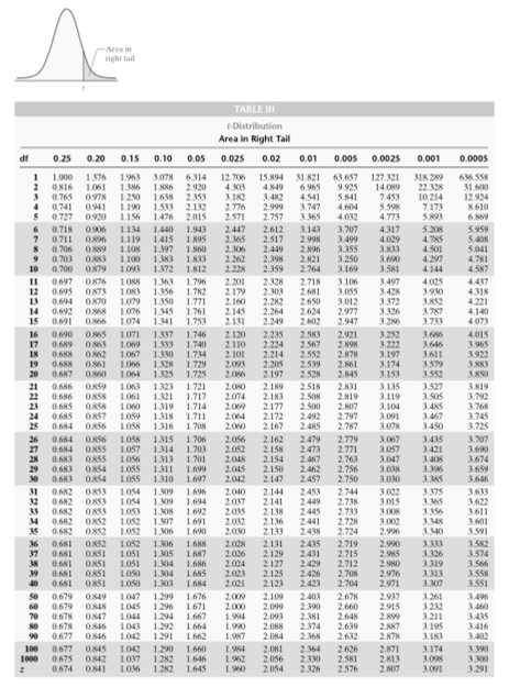
of various sample sizes. A new table:
Below is the new t table that is in the foldout in the back of your book. I
gave a copy of it out in class for reference. This new table makes
adjustments to the normal curve based on the sample size. The df in the upper
left-hand corner of the table is the “degrees of freedom”. The df is one less
than the sample size, i.e., df=n-1. This n-1 is the same correction factor
that you saw in the computation for s way back at the beginning of the
semester:
Note that the top row and
the bottom row have the numbers you were using in the abbreviated table for
looking up critical values for z tests.
To use the new part of the
table, you take one less than the sample size, df=n-1 and go down to that row
instead of down to the bottom where the z values lie. Use the table
symmetrically so that it works for negative t values and gives areas in the
left tail of the distribution also. EXAMPLES USING THE t-TABLE TO FIND CRITICAL VALUES
AND P-VALUE ESTIMATES: 1. What is the
critical value for a one-sided test with n=20 and alpha =0.05? ANSWER: df=20-1=19 and that row put together
with the column of 0.05 gives a critical value of 1.729 2. What would
the critical value be for the above situation if it were two-sided instead of
one-sided? ANSWER: In the same row df=19, you would look at
the column with area 0.025, since half of the alpha of 0.05 goes into each
tail, and this would give you a critical value of 2.093. 3.
Find an estimate for
the p value in a one-sided test with n=33 and sample t=0.52. ANSWER: df=33-1=32, so we look in that row on
the new t table to find the next higher and lower numbers with respect to
0.52. But since 0.52 < 0.682 the p value then is greater than the area of
0.25 for the t value of 0.682. That is, p > 0.25. 4. Find an
estimate for the p value for a two-sided test with n=25 and sample t value of
1.52. ANSWER: df=25-1=24 and in that row, 1.318 <
1.52 < 1.711 so the right or left tail area for the p value is between
0.10 and 0.05, but we have a two-sided test so we double the areas to get the
sum of the left and right tail areas: 0.10 < p < 0.20. HOMEWORK DUE TUESDAY 10/12 (read
the examples above and in the book first!): 1. 10.3 p487 #6 2. 10.3 p487
#10 3. 10.3 p487
#12 4. 10.3 p488
#16 5. 10.3 p488
#20 (do part a and skip part b) |
||||||||||||||||||||||||||||||||||||||||||||||||||||||||||||||||||||||||||||||||||||||||||||||||||||||||||||||||||||||||
|
T 10/05 |
We worked on the whole
significance test in class today. This is the material from section 10.2 in
your book. Look at the examples in the section and the following additional
examples: Example: Grant is in the market to
buy a three-year-old Corvette. Before shopping for the car, he wants to
determine what he should expect to pay. According to the blue book, the
average price of such a car is $37,500. Grant thinks it is different from
this price in his neighborhood, so he visits 15 neighborhood dealers online
and finds and average price of $38,246.90. Assuming a population std.
deviation of $4100, test his claim at the 0.10 level of significance. Hypotheses: Ho: population mean =
37500 Hi: population mean not equal to 37500 Level of
Significance: alpha = 0.10 Data and
calculations: z = (38246.90 - 37500)/(4100/sqroot15) = 0.71 Decision: Method 1: For 0.05 of alpha
going in each tail, we find a critical z value of 1.645 and the sample z is
not as far out from the theoretical population mean. Method 2: Look up sample
z of 0.71 on the abbreviated table and find 0.674 < 0.71 < 0.841 so
2(0.25) > p > 2(0.20), that is, the p value is between 40 and 50 %,
whereas the alpha was 10%. By either method, we find that we do not have
evidence to reject the null hypothesis, so we accept it. Conclusion: Grant does not have any
evidence that the mean price of a 3 yr. old Corvette is different
from $37,500 in his neighborhood. Example: According to the U.S.
Federal Highway Administration, the mean number of miles driven annually in
1990 was 10,300. Bob believes that people are driving more today than in 1990
and obtains a simple random sample of 20 people and asks them the number of
miles they drove last year. Their responses give an average of 12,342 miles.
Assuming a std. deviation of 3500 miles, test Bob’s claim at the 0.01 level
of significance. Hypotheses: Ho: population mean = 10300 Hi: population mean > 10300 Level of
Significance: alpha = 0.01 Data and
calculations: Z=(12342-10300)/(3500/sqroot20)=2.61 Decision: The alternate hypothesis is one-sided on the right, the
sample z works out to be 2.61, and we reject the null hypothesis. (Method 1: alpha of 0.01 gives a critical z
value of 2.326 and 2.61 is farther out than that. Method 2: on the
abbreviated table for critical values, we look up 2.576 <2.61<2.807 and
find an estimated p value of 0.005 > p > 0.0025 which is less than the
alpha of 0.01. By either of these methods, we reject the null hypothesis). Conclusion: Bob has found significant evidence that people are
driving more today than in 1990, when they drove an average of 10,300 miles. Homework due Thursday 10/07: For each of the
following word problems, perform a complete significance test with: --Hypotheses
(null and alternate), --Level of
significance (given in problem), --Sample z
calculation, --Decision to
accept or reject the null hypothesis (show using both methods) --Sentence of
conclusion relating back to the original problem. 1. section 10.2
p468/469 redo ex. 2 with everything the same except the sample mean is 53.75
instead of 65.014. 2. section 10.2
p476 #20 3. section 10.2
p478 #30 4. section 10.2
p478 #32 5. section 10.2
p478 redo #32 with everything the same except the sample mean is 7.8 instead
of 13.3. |
||||||||||||||||||||||||||||||||||||||||||||||||||||||||||||||||||||||||||||||||||||||||||||||||||||||||||||||||||||||||
|
Th 09/30 |
We have talked about what the level of significance is and how it is used, how to find the z value calculation using the sample data, and how to make a decision to accept or reject Ho. We need to talk about how to state the hypotheses from word problems and how to write the sentence of conclusion. Before the
test, I briefly talked about these hypotheses that come from a word problem
such as those in section 10.2. I would also like you to try writing sentences
of conclusion (we did not have time for that before the test). Some examples
follow below.
HYPOTHESES:
The null hypothesis, symbolized by Ho is what is accepted as true for the population mean until evidence to the contrary is found.
The alternate hypothesis, symbolized by H1 is what the investigator or researcher is trying to show (always relating to the number for M used in the null hypothesis). The choice of an appropriate alternative hypothesis depends on what we hope to be able to show as evidence against accepting the null hypothesis. As we start work on word problems, it is important that you form alternate hypotheses based on the intent of the investigator in the problem.
CONCLUSION:
You must state what you have found from the sample’s evidence, or lack thereof. Write a grammatically complete sentence with the following elements: Tell
1. if you have “found evidence” or “not found evidence” against the null hypothesis, 2. about what (what was the subject of the investigation?), 3. with respect to what number (what was the number in question in the hypotheses?).
If you are rejecting the null hypothesis, you have found evidence against the null hypothesis and therefore evidence for your claim in the alternate hypothesis. If you are accepting the null hypothesis, you have not found evidence against it and therefore have not found evidence to back up your claim in the alternate hypothesis.
Here are a few word problem examples on how to write the hypotheses and sentences of conclusion:
Example: An energy official claims that the output of oil per well in the US has increased from the 1998 level of 11.1 barrels per day. Suppose that after she takes a random sample and calculates the sample z value she decides to reject the null hypothesis Ho. Write the hypotheses and the sentence of conclusion. Answer: H0 : M =11.1 H1 : M >11.1 The energy official has found evidence that the output of oil per well in the U. S. has increased significantly from the 1998 level of 11.1 barrels per day.
Example: A Muni bus drives a prescribed route and the supervisor wants to know whether the average run arrival time for buses on this route is about every 28 minutes. Suppose that after we calculate the sample z value the data causes the supervisor to accept the null hypothesis. Write the hypotheses and the sentence of conclusion. Answer: H0 : M = 28 H1 : M is not equal to 28 The supervisor has found no evidence that the average run arrival time for buses on this route is significantly different from 28 minutes.
Example: A manufacturer produces a paint which takes 20 minutes to dry. He wants make changes in the composition to get nicer colors, but not if it increases the drying time needed. Suppose that after he calculates the sample z value the data causes him to reject the null hypothesis. Write the hypotheses and the sentence of conclusion. Answer: H0 : M = 20 H1 : M > 20 The manufacturer has found evidence that the composition change significantly increases the drying time, so he will not make a change. (Notice that he is using the test to pull him away from a bad decision).
HOMEWORK (due Tuesday 10/05): Read section 10.1 in the text, which is about how to form appropriate null and alternate hypotheses from word problems and write a sentence for the indicated conclusion (no calculations or accept/reject tests are needed here!). Then do the following for homework: 10.1 p460/461 (the first three groups are paired problems involving the same situation): #16 a.(state hypotheses do not do b. about error type) and 24 (write sentence of conclusion), #18 a.(state hypotheses do not do b. about error type) and 26 (write sentence of conclusion), #20 a. (state hypotheses do not do b. about error type) and 28 (write sentence of conclusion), #36 a, b (do not do c) #38 a, b (do not do c) |
||||||||||||||||||||||||||||||||||||||||||||||||||||||||||||||||||||||||||||||||||||||||||||||||||||||||||||||||||||||||
|
T 09/28 |
Test #2 will occur as
scheduled on Thursday 09/30. It will cover how critical values are found, the
effect of making changes to confidence levels, sample size, etc., word
problems using formulas (given) for confidence, error, and sample size, use
of critical values and p-values to accept and reject hypotheses, and
computation of z values using the formula (given). Homework is to study for
your test. I put a few more hmk/quiz papers outside my office BH269 if you
want to pick them up to help you study. |
||||||||||||||||||||||||||||||||||||||||||||||||||||||||||||||||||||||||||||||||||||||||||||||||||||||||||||||||||||||||
|
Th 09/23 |
More DECISION MAKING in significance tests: We talked today about another method to reject and accept the null hypothesis, other than finding critical values. This is talked about in the text on p469-473. It involves using the abbreviated table to make estimates of the likelihood of getting a certain sample z value. The “p-value” area is the probability that you would get a value as far away or farther away from the center as the sample value you got. Your goal is then to compare the alpha area with the p-value area. This will be an important method as we go forward into the world of significance tests. Especially important since you do not even necessarily have to have an alpha value to compare with the p value You might just be able to make a statement of likelihood of the sample value occurring in a normal distribution, and this might make or break the case against the null hypothesis without comparison to an alpha value. The following are the some examples using this new method.
We find an estimate for the p value using the quick reference chart for finding critical values:
Some examples: 1. Ho : M =54.3 H1 M < 54.3 alpha= 0.01 sample z=-2.10 Estimating p: looking at the above table, we see that our sample is between the critical values of 2.054 and 2.326 whose tail areas are at the top of the table, 0.02 and 0.01 respectively. So we know that the p value area for our sample is between these critical areas. If p is between 0.02 and 0.01, but not equal to them, we know that p is greater than the alpha of 0.01 given, so we accept the null hypothesis. 2. Ho : M = 6 H1 : M not equal to 6 alpha= 0.02 sample z= 2.40 Estimating p: looking at the above table, we see that our sample is between the critical values of 2.326 and 2.576 whose right or left tail areas are 0.01 and 0.005 respectively. Since the alternate hypothesis is two-sided, we are also interested in the areas of the other tail which are the same, 0.01 to 0.005. So we know that the p value area for our sample is between the sum of these critical areas, that is, 0.02 and 0.01. If p is between 0.02 and 0.01, but not equal to them, we know that p is less than the alpha of 0.02 given, so we reject the null hypothesis. 3. Ho : M = 40 H1 : M > 40 alpha= 0.05 sample z= 1.52 Estimating p: looking at the above table, we see that our sample is between the critical values of 1.282 and 1.645 whose tail areas are at the top of the table, 0.10 and 0.05 respectively. So we know that the p value area for our sample is between these critical areas. If p is between 0.10 and 0.05, but not equal to them, we know that p is greater than the alpha of 0.05 given, so we accept the null hypothesis. 4. Ho: M = 23 H1 : M not equal to 23 alpha= 0.10 sample z= -1.5 Estimating p: looking at the above table,
we see that our sample is between the critical values of 1.282 and 1.645
whose right or left tail areas are at the top of the table, 0.10 and 0.05
respectively. Since the alternate hypothesis is two-sided, we are also
interested in the other tail area which is the same, 0.10 to 0.05. So we know
that the p value area for our sample is between the sum of these critical
areas, that is, 0.20 and 0.10. If p is between 0.20 and 0.10 but not equal to
them, we know that p is greater than the alpha of 0.10 given, so we accept the null hypothesis. You do not always have to find upper and lower bounds for the p-value: 5. Ho : M = 120 H1 : M > 120 alpha= 0.05 sample z= 3.35 Estimating p: looking at the above table, we see that our sample is not between any critical values, but is larger than the largest critical value on the table: 3.291. That means that the p value for the sample z must be smaller than the smallest area in the table (which is the tail area above 3.291). So we know that the p value area for our sample is smaller than 0.0005. That means that our sample is very rare for the center of the distribution to be at 120, which was claimed in the null hypothesis. So even without an alpha given, we would know that it is very unlikely that the null hypothesis is correct, so we reject the null hypothesis based on this very persuasive evidence. But also, whenever the p value is less than the alpha value, you reject the null hypothesis. 6. Ho : M = 16 H1 : M not equal to 16 alpha= 0.01 sample z= 0.45 Estimating p: looking at the above table,
we see that our sample is not between any critical values, but is smaller
than the smallest critical value on the table: 0.674. That means that the p
value for the sample z must be larger than the largest area in the table
(which is the tail area above 0.674). So we know that the p value area for
our sample is larger than 0.25+0.25=0.50 (doubled because the alternate
hypothesis is two-sided). That means that our sample is very common for the
center of the distribution to be at 16, which was claimed in the null
hypothesis. So even without an alpha given, we would know that we have come
nowhere near to finding any evidence against the null hypothesis, so we accept the null hypothesis based on
this very unpersuasive evidence. But also, whenever the p value is more than
the alpha value, you accept the null hypothesis. Homework due Tuesday 09/28: Give the above process a
try in the book problems 10.2 p476 that you did last time, but now do all
using the p-value method for all. See that you get the same answers as you
did using the critical value method. No pictures are required for this
method. Just tell how you are estimating the p values using the abbreviated
table values. 12. use sample z = 1.92 13. use sample z = 3.29 14. use sample z =
–1.32 16. use sample z = 1.20 17. use sample z =
–1.87 You will have a test next
Thursday. It will cover how critical values are found, the effect of making
changes to confidence levels, sample size, etc., word problems using formulas
for confidence, error, and sample size, and use of critical values and
p-values to accept and reject hypotheses. Possibly computation of z values
using the formula will be included. I will let you know on Tuesday. |
||||||||||||||||||||||||||||||||||||||||||||||||||||||||||||||||||||||||||||||||||||||||||||||||||||||||||||||||||||||||
|
T 09/21 |
Some supplement to your reading with a few more examples: Today we started looking at how to make a DECISION, given the hypotheses, level of significance and the z value already calculated, since the decision phase is logically the hardest part of the significance test to understand. Later, after we have mastered the techniques of decision making, then we will look at word problems involving the whole process of significance tests! Sorry, but I cannot reproduce pictures of the normal distribution here, but you should draw one for each problem, with shaded areas of rejection and critical values!
I gave a handout with some sample problems in class, and included on it was the following abbreviated table of critical values, so you do not have to look them up on the old table backwards each time you want to do a problem. The top row represents the area in either the left or right tail of the distribution, and the bottom row represents the positive or negative critical value, depending on which tail you are looking at. Refer to it as you look at the example problems below:
Example of “two-sided” significance tests:
If the null hypothesis is that the mean of a population is 35 and the alternate hypothesis is that the mean of the population is not 35 (within a certain amount of acceptable error) and a level of significance is given as 0.02 and you take a sample and standardize it to get z= 2.20, does it give enough evidence to reject the null hypothesis and therefore accept the alternate hypothesis? Answer: One way of determination is to compare the sample z to the critical value of z. The critical values come from the alpha value. That is, if you look up an area of alpha 0.02 (level of significance) divided by 2 to get 0.01 (this is how much goes in each tail of the distribution) on the table above, you see a critical z* of +/–2.326. Since the sample z of 2.20 is closer to the mean than 2.326 you have no evidence to reject the null hypothesis, so you must Accept it.
Example of “one-sided” significance tests:
If the null hypothesis is that the mean of a population is 365 and the alternate hypothesis is that the mean is greater than 365 and alpha=0.02, sample z=2.73 Answer:
Alpha goes into the right tail and the z that marks the spot such that there
is 0.02 to its right is 2.054 using the abbreviated table at the top of these
notes. Since our sample z of 2.73 is farther away from center than 2.054, we Reject the null hypothesis. Homework due Thursday 09/23: Give the above process a
try in the book problems 10.2 p476 with the following directions: Draw a separate normal
distribution for each and label relevant z values and areas (refer to table
above for critical values). Note that #15-18 ask you to use the p-value
method which we will talk about on Thursday. For now, just use the critical
value method for all of the below problems. 12. use sample z = 1.92 for
part a, then do parts b, c, d 13. use sample z = 3.29 for
part a, then do parts b, c, d 14. use sample z =
–1.32 for part a, then do parts b, c, d 16. use sample z = 1.20 for
part a, then do as in parts b, c, d in #11-14, with alpha = 0.10 17. use sample z =
–1.87 for part a, then do as parts b, c, d in #11-14, with alpha = 0.02 |
||||||||||||||||||||||||||||||||||||||||||||||||||||||||||||||||||||||||||||||||||||||||||||||||||||||||||||||||||||||||
|
Th 09/16 |
We worked with confidence,
error, and sample size again today. If you want to start reading ahead for
next week, we will begin looking at hypothesis tests in ch 10. This is a
rather involved process, and we will spend the coming weeks building it up a
little at a time. You might want to prepare by reading: 10.1 objective 1 on p 454 to 456 (determine the null and alternate hypotheses), 10.2 objective 1 on p462 to
465 (understand the logic of hypothesis testing). Note that 10.2 p467 to p469 examples 1 and 2 show the whole process of a significance test, and it is good to scan through them so you get an idea of what’s to come, but don’t worry too much about the details yet! On Tuesday, we will only
work on steps 4 and 5 of the process, which are summarized on p466 and
p469/470 in the blue boxes. This is the most difficult part of the process.
Once it is understood, then we can start putting the whole test strategy
together! Homework due Tuesday 09/21: 1. In the text, 9.1 p417 #24
2. In the text, 9.1 p420 # 40
3. Supplemental problem to the text: A random sample of 300 telephone calls made to the office of a large corporation is timed and reveals that the average call is 6.48 minutes long. Assume a std. deviation of 1.92 minutes can be used. If 6.48 minutes is used as an estimate of the true length of telephone calls made to the office, a. What can the office manager say with 99% confidence about the maximum error? b. What can the office manager say with 90% confidence about the maximum error?
4. In the text, 9.1 p420 #36 the answer to part a is x bar (the sample mean) is 40520.2 miles. Using this info, do parts b, c, and d.
5. Supplemental problem to the text: A large hospital finds that in 50 randomly selected days it had, on average 96.4 patient admissions per day. From previous studies it has been determined that a population std. deviation of 12.2 days can be used. Using a 90% confidence level, a. How large a sample of days must we choose in order to ensure that our estimate of the actual daily number of hospital admissions is off by no more than five admissions per day? b. How large a sample of
days must we choose in order to have 25% of the error we had in part a? |
||||||||||||||||||||||||||||||||||||||||||||||||||||||||||||||||||||||||||||||||||||||||||||||||||||||||||||||||||||||||
|
T 09/14 |
Before doing the problems
below, try to read some of the material in 9.1 in the text: p405-406 thinking about +/-
error p409 bottom: see the recap
of critical values for 90/95/99% confidence p407-411 constructing a
confidence interval (especially ex. 3 p411) p412-413 error formula
(especially ex. 5/6 on p413) p413-414 sample size
formula (especially ex. 7 on p414) Read 9.1 p416 #17, try it
and look at the answers in the back of the book. Homework due Thursday 09/16: Make note for yourself in
comparing the parts to a problem how changes in confidence and sample size
affect error and interval width. In your work below, use the answers 9.1 p416 #13 answer 2.33
#14 answer 1.88 #15 answer 1.44
#16 answer 1.28 and round error and confidence interval values to 2 decimal places. Turn in: 1. 9.1 p416 # 18 parts a, b, c (skip part d) 2. 9.1 p416 # 20 parts a, b, c (skip parts d and e) 3. 9.1 p417 #26 parts c, d, e using sample mean of 103.4 and n=9 (skip parts a and b) 4. 9.1 p420 #38 (use the
formula for sample size with E = 1.5) 5. 9.1 p420 #42 parts a, b, c |
||||||||||||||||||||||||||||||||||||||||||||||||||||||||||||||||||||||||||||||||||||||||||||||||||||||||||||||||||||||||
|
Th 09/09 |
Before starting Test #1, I
asked you to think about the sampling distribution (ch 8) and using the table
backwards to find z values if you are given a certain amount of area in the
middle of the distribution (a confidence level, ch.9). We call the z values that
mark a predetermined area in the center “critical values”, which I will
denote by z*. We call the area in the center of the distribution the confidence level. As another example like the
one in class, find the z* for the confidence level of 85%. Answer:
Since this area is in the middle of the distribution about the mean (42.5%
directly to the right and left of center), 1-85% or 15% is outside of this
center range, so 7.5% area is in each tail of the distribution. The closest
area in the table to 7.5% or 0.075 is 0.0749 which gives a z value of
–1.44. So the z* are –1.44 and +1.44 (positive and negative
values mark each tail on either side of the mean). Read about the sampling
distribution in section 8.1 and see how the new z calculation is made in ex4
p 383 and ex. 6 p387. I suggest that you may calculate the value in the
following way to avoid errors, by multiplying by the reciprocal of the
fraction in the denominator instead of dividing by it: For example, if the mean of
the population is 12.7, the std. deviation of the population is 2.5, the
sample size is 5, and the sample mean is 12.5,
HOMEWORK
(due on Tuesday): Find the critical values for the following situations
(make and label a picture for each): 1. If you have a confidence level of 88%, what are
the z* critical values? 2. If you have a confidence level of 90%, what are
the z* critical values? 3. If you have a confidence level of 95%, what are
the z* critical values? 4. If you have a confidence level of 99%, what are
the z* critical values? Use the new z formula for the sampling distribution: 5. Find z if the mean of the population is 45.7, the
std. deviation of the population is 13.2, the sample size is 75, and the
sample mean is 48.2. |
||||||||||||||||||||||||||||||||||||||||||||||||||||||||||||||||||||||||||||||||||||||||||||||||||||||||||||||||||||||||
|
T 09/07 |
We did not get to any new
material today, as we went over hmk and did a few more problems of those
types. Homework is to study for your test. Test #1 will occur as
scheduled on Thursday 09/09. Please remember to bring a
standard calculator (not a cell phone/texting/PDA device). You will be given the
formulas for std. deviation (s) and for finding std. scores (z). You will
also be given a copy of the z-table (symmetric one-page version) with your
test. Your test paper will have room on it for you to work the problems. The test will include
problems like those we have worked on in our 5 class sessions so far: Finding the mean and std.
deviation of data (by finding squared deviations and using the formula). Possibly some short answer
questions about finding and interpreting areas. A standard scores
comparison word problem (as in last hmk’s #4 and 5 from section 3.4). Several normal distribution
word problems (as in last hmk’s #1-3, etc.) to demonstrate “forwards” and
“backwards” techniques – some will have linked parts or related
follow-up questions. Look at the class notes,
hmk, quizzes and see the book for more examples: 3.1 p107-109 mean 3.2 p125-132 standard
deviation and empirical rule 3.4 p150 comparing z-scores (standardized scores) 7.1 p319-327 standardizing formula and area under the normal curve 7.2 p331-341 finding area under the normal curve (be careful that we a using a modified version of the table in the book—the table in the book has separate +/- values, but the answers to the area exercises should ultimately come out the same) 7.3 p345349 word problems using the standard normal curve. You will have one hour to
complete the test. In the 15 minutes or so before the test, I will describe
some homework that I would like for you to complete. It will be related to
the work we have been doing, but will help to prepare us for the material for
next week. |
||||||||||||||||||||||||||||||||||||||||||||||||||||||||||||||||||||||||||||||||||||||||||||||||||||||||||||||||||||||||
|
Th 09/02 |
We went over the hmk and
moved on to 3.4 p150 like ex.1: comparing z-scores. You have more hmk on
normal curve word problems and some std. score problems from 3.4 due Tuesday.
We will finish up details of some new material on Tuesday, then you have your
first scheduled test on Thursday 09/09. Homework due Tuesday 09/07: Problems 1, 2, 3 are like those
you find in section 7.3 (see the section for more examples and problems to
try for practice). Problems 4 and 5 are from section 3.4. 1. The number of days that patients are hospitalized is on average 7.1 days with std. deviation of 3.2 days. How many days do the 20% longest-staying patients stay?
2. The average amount of radiation to which a person is exposed while flying by jet across the U.S. is 4.35 units with std. deviation of 3.2. What is the probability that a passenger will be exposed to more than 4 units of radiation?
3. In the radiation problem above, below what number of units of radiation lie the 15% of passengers that receive the smallest amount of radiation? 4. (from 3.4 p157 #10) The average 20-29-year-old
man is 69.6 inches tall, with a std. deviation of 2.7 inches, while the
aerage 20-29-year-old woman is 64.1 inches tall, with a std. deviation of 2.6
inches. Who is relatively taller, a 68-inch man or a 62-inch woman? 5. (from 3.4 p157 #12) The highest batting average
ever recorded was by Ted Williams in 1941 when he hit 0.406. That year, the
mean and std. deviation for batting average were 0.28062 and 0.03281. In
2004, Ichiro Suzuki was the American League batting champion, with a batting
average of 0.372. In 2004, the mean and std. deviation for batting average
were 0.26992 and 0.02154. Who had the better year relative to their peers,
Williams or Suzuki? |
||||||||||||||||||||||||||||||||||||||||||||||||||||||||||||||||||||||||||||||||||||||||||||||||||||||||||||||||||||||||
|
T 08/31 |
I am putting notes and homework here again because some of you may not have received your book yet if you ordered it last week. However, by Thursday, I will start assigning work from the book. For those who have the book, so far we have looked at the following: 3.1 p107-109 mean 3.2 p125-132 standard deviation and empirical rule 7.1 p319-327 standardizing formula and area under the normal curve 7.2 p331-341 finding area under the normal curve (be careful that we a using a modified version of the table in the book—the table in the book has separate +/- values, but the answers to the area exercises should ultimately come out the same) 7.3 p345349 word problems using the standard normal curve. Although the notes provided below contained most of what was needed from these sections and contained more detailed examples, going back to read these sections and trying some of the problems in them can help your understanding, especially if you missed class.
NOTES
In a “forwards” direction problem, you are given an x value (or two x values) and use the standardizing formula z = ( x – mean)/(std. deviation) to find the z value(s) that counts the number of std. deviations that the x value lies from the mean. Then you use the z value to look up the area in the tail of the distribution corresponding to the original x value or further away from the mean.
EXAMPLE (similar to the “forwards” problem from #3 of the class exercises): In an experiment to determine the amount of time required to assemble an "easy to assemble” toy, the average time to assemble it was 27.8 minutes with a standard deviation of 4.0 minutes. What is the probability that a randomly selected person will assemble the toy in more than 30 minutes? Answer: You want to find the area under the curve corresponding to x values more than 25. When x=30, z= (30-27.8)/4= 0.55. We use this standardized value of x to look up the area under the curve. On the table, this z value gives an area of 0.2912. Since this is the area for values more than 30 ( to the right of 30) this is our answer. About 29% of the time one would expect a person to assemble the toy in more than 30 minutes.
EXAMPLE (similar to the “forwards” problem from #2 of the class exercises): A salesman has an average car route trip time of 4.3 hours with std. deviation of 0.2 hours. What is the probability that the length of his car trip will last anywhere from 4 to 4.5 hours? Answer: For x=4, z=(4-4.3)/0.2=-1.5 and for x=4.5. z=(4.5-4.3)/0.2=1.0. The area to the left of –1.5 is 0.0668 and the area to the right of 1.0 is 0.1587. The area between is 1-(0.1587+0.0668)=0.7745, so there is about a 77% chance that his trip will last anywhere from 4 to 4.5 hours.
Some word problems are harder because you are given an area that represents the probability of a certain event or that is a percentage or proportion of a distribution, and have to find an x value that marks the spot where that area begins. I refer to these as “backwards” problems: In “backwards” problems, you use the process in the “forwards” problems, but in the reverse direction. You start by identifying the given area in a picture and use the table of areas to find the z value that corresponds to it. Look in the middle of the table for the closest area to the one you are given, map it backwards to find the row and column it belongs to in order to find the z value, then take the resulting z value and “unstandardize” it (solve for x) in the formula z = ( x – mean)/(std. deviation)! Consider the following examples of “backwards” problems:
EXAMPLE (“backwards” problem using a variation of #1 from in-class exercises): The average assembly time was 27.8 minutes with a standard deviation of 4.0 minutes. Above what number of minutes lie the 25% slowest assembly times? Answer: This is a “backwards” problem since you are looking for an x value (number of minutes), having been given an area. You are given the area of 25% which as a decimal is 0.25, and the closest value to this in the table is 0.2514. Looking from this area to what row and column it belongs to, we see this area corresponds to a z value of +0.67. This is a z value on the right side of the distribution since the “slowest” assembly times involve the most number of minutes, and these occur in the right side of the distribution, where the average time of 27.8 is in the middle. Here is a case where the wording in the problem might not match your intuition! The right-hand side of the distribution does not necessarily represent the biggest, strongest, fastest numbers. It depends on the situation. Now we “unstandardize” this value by using the formula to solve for x : +0.67=(x-27.8)/4.0 so x=(+0.67)(4.0)+27.8=30.48 or about 30 minutes. The 25% slowest assembly times take about 30 or more minutes. (almost the same as the previous “forwards” version of the problem).
EXAMPLE (very much like “backwards” problem #4 from in-class exercises): In a very large world history class, the final exam grades have a mean of 66.5 and a standard deviation of 12.6. Above what score lie the highest 25% of the scores? Answer: This is a “backwards” problem since you are looking for an x value, having been given an area. You are given the area of 0.25, so draw this area as a right tail in the distribution since the highest scores in the class are to the right of the mean (the average score is in the center). The closest value to 0.25 in the table is 0.2514. This area corresponds to a z value of +0.67 (note that the one in class was negative!). This is a positive z value since the higher grades are in the right side of the distribution. You will not get the correct answer if you do not include the correct sign of the z value. We “unstandardize” this value by using the formula to solve for x and get +0.67=(x-66.5)/12.6 so x=(+0.67)(12.6)+66.5=74.942. About 25% of the class had scores of 74.9 or higher.
EXAMPLE (somewhat like “backwards” problem #5 from in-class exercises): The lengths of sardines received by a cannery have a mean of 4.64 inches and a standard deviation of 0.25 inches. If the distribution of these lengths can be approximated closely with a normal distribution, below which length lie the shortest 18% of the sardines? Answer: This is a “backwards” problem since you are looking for an x value (length of sardines), having been given an area. You are given the area of 0.18, which is a left-hand tail in the distribution, because it represents below-average lengths. The closest value to this in the table is 0.1814. This area corresponds to a z value of – 0.91. We “unstandardize” this value by using the formula to solve for x and get – 0.91=(x-4.64)/0.25 so x=(– 0.91)(0.25)+4.64= –0.2275+4.64=4.41. About 18% of the sardines measure 4.4 inches or shorter.
EXAMPLE (“backwards” problem using a variation of #1 from in-class exercises): The average assembly time was 27.8 minutes with a standard deviation of 4.0 minutes. Above what number of minutes lie the 60% slowest assembly times? Answer: This is a “backwards” problem since you are looking for an x value (number of minutes), having been given an area. You are given the area of 60% which as a decimal is 0.60, but you can only find areas from 0% to 50% on the table! To find an area of 60% above an x value, the x value must be to the left of the mean. So you must use the area to the left of this x value, which is 40%, or 0.40. The closest value to 0.40 in the table is 0.4013. Looking from this area to what row and column it belongs to, we see this area corresponds to a z value of –0.25. This is a z value on the left side of the distribution, so it is negative. Now we “unstandardize” this value by using the formula to solve for x : –0.25=(x-27.8)/4.0 so x=(–0.25)(4.0)+27.8=26.8 minutes. The 60% slowest assembly times take about 26.8 or more minutes.
HOMEWORK WORD PROBLEMS (due Thursday 09/02): Note that you should provide a picture with x, z and area values for all of the problems below, and try writing a brief sentence of conclusion as in the above examples.
1. In an experiment to determine the amount of time required to assemble an "easy to assemble” toy, the average time to assemble it was 27.8 minutes with a standard deviation of 4.0 minutes. What is the probability that a randomly selected person will assemble the toy in anywhere from 30 to 35 minutes?
2. In a very large world history class, the final exam grades have a mean of 66.5 and a standard deviation of 12.6., what percent of the class should receive an A if A’s are given to those with scores of 87 or better? Follow-up question: If there were 720 students in this large lecture class, how many students received an A?
3. John’s Homemade Dressing has an average of 8.5 ounces of dressing per bottle with a std. deviation of 0.5 ounces. Above what number of ounces can one find the 30% most-over-filled bottles?
4. For a salesman driving between cities, the average trip time is 4.3 hours with std. deviation of 0.2 hours. Below what time lie the fastest 20% of his trips? (Be sure you think about what a “fast” trip is! Where are the fastest trips in the distribution?).
5. For the history class problem above in #3, with mean of 66.5 and std. deviation of 12.6. Sixty-five percent of the scores lie above what score? (Tricky! 65% is more than half of the distribution. To be able to have 65% above a score, where in the distribution should the score be?).
|
||||||||||||||||||||||||||||||||||||||||||||||||||||||||||||||||||||||||||||||||||||||||||||||||||||||||||||||||||||||||
|
Th 08/26 |
Once you know how to calculate the mean and standard deviation for a normal distribution, you can put these two important numbers to work to “standardize” any normal distribution. We convert a particular score in the distribution into a standardized z score by way of the following:
Some problems to practice finding standardized (z) values (not to turn in):
1. What if a normal distribution has a mean of 80 and a standard deviation of 10, what is the z value for each of the following (use the formula for z given above): a. 110 Answer: z=(110-80)/10=3 b. 80 Answer: z=(80-80)/10=0 (the mean always standardizes to 0!) c. 60 Answer: z=(60-80)/10= -2 d. 65 Answer: z=(65-80)/10= -1.5
2. What if a normal distribution has a mean of 63.2 and a standard deviation of 7.8, find the z value for each using the formula: a. 63.2 Answer: z=(63.2-63.2)/7.8=0 b. 58.9 Answer: z=(58.9-63.2)/7.8= -0.55 c. 67.5 Answer: z=(67.5-63.2)/7.8=+0.55 (symmetry with part b!) d. 64.8 Answer: z=(64.8-63.2)/7.8= 0.205128205.... = 0.21 (round to 2 places!)
I gave you a copy of the table below in class today. The z table gives the areas under the std. normal curve for particular z scores. We will use a modified version of this table (which cannot be readily represented here), where we employ the symmetry of the curve so that the area to the left of a negative z value is the same as the area to the right of a positive z value. In that way, you can look up the z values below as + or – instead of just –.
To look up a particular value of z, you put together the row and column that make up the z value. The left-most column gives the ones and tenths places of the z, but the uppermost row gives the hundredths place of the z value. For instance, if the z value is 1.83, since 1.83=1.8+0.03, you look to the row of 1.8 and the column of 0.03 to find the area under the curve : 0.0336. Examples: 1. What is the area under the standard normal curve for values to the left of z= -1.57 Answer: Putting row 1.5 with column 0.07 we get 0.0582 2. What is the area under the standard normal curve for values to the right of z= 2.02? Answer: Putting row 2.0 with column 0.02 we get 0.0217
Remember that we convert the original normal distribution made up of x data values into the standard normal distribution of z values using the standardizing formula. We do this in order to be able to look up the area under the curve for a given value using the table. When you work on these problems involving areas under the normal curve, draw a normal curve and fill in the numbers of interest for a particular problem on number lines below the curve: one number line for the unstandardized original data (the x data points), and one number line for the standardized values (z values for each given x, found using the standardizing formula, that correspond to the standard normal curve for which we have a table to look up areas). Once you have all known values on your picture, think about what area under the curve you are looking for and what areas you have from the table for the z values of interest. Then you must decide how to use the table values to find the area you need, and this may not be immediately apparent!
Practice problems (not to turn in) using the table to look up areas under the standard normal curve (where the standardized value z has already been found from some given data):
1. What is the area to the left of z= -1.75 Answer: 0.0401 2. What is the area to the left of z= -2.04? Answer: 0.0207 3. What is the area to the right of z=2.79? Answer: 0.0026 4. What is the area to the right of z=1.05? Answer: 0.1469 5. What is the area to the left of z= -0.06? Answer: 0.4761 6. What is the area to the left of z= -0.60? Answer: 0.2743 7. What is the area to the right of z= 0.60? Answer: 0.2743 8. What is the area to the right of z= -1.74? Answer: 0.9591 (from 1-0.0409) 9. What is the area to the left of z=1.05? Answer: 0.8531 (from 1-0.1469) 10. What is the area to the left of z=1.50? Answer: 0.9332 (from 1-0.0668) 11. What is the area to the right of z= -2.17? Answer: 0.9850 (from 1-0.0150) 12. What is the area to the right of z= -0.05? Answer: 0.5199 (from 1-0.4801) 13. What is the area to the left of z= 3.33? Answer: 0.9996 (from 1-0.0004) 14. What is the area to the right of z= 0.67? Answer: 0.7486 (from 1-0.2514) 15. What is the area between z=0.87 and z=2.03? Answer: 0.1710 (The smaller tail corresponding to z=2.03 has area of 0.0212 and the larger tail corresponding to z=0.87 has area of 0.1922. The smaller tail area, though, is contained within the larger tail area, so that if you want the area between them, you must take the larger and subtract the smaller: 0.1922-0.0212=0.1710) 16. What is the area between z= -0.25 and z= -1.97 Answer: 0.3769 (Same as the above, subtract the smaller tail from the larger tail: 0.4013-0.0244 = 0.3769) 17. What is the area between z= -2.09 and z=3.07? Answer: 0.9806 (This is different from the previous two problems, because the values are on opposite sides of the distribution and so it is not the case that one tail is contained within the other. You must start with 100% of the whole distribution and “chop off” the two tails using subtraction: 1-(0.0183+0.0011) or 1-0.0183-0.0011 which equals 0.9806)
Practice problems (not to turn in) to convert word problems to pictures, z values, and areas (Due to limited capabilities of this website, I cannot draw a picture in here like those we did in class, but you should! Look at the curve above the table of z values above, draw one for each problem, with one horizontal number line below the curve for the original x data values and one below that for the standardized z values):
Suppose a large group of students took a test (the results are distributed normally), and suppose that the average score was 73 with std. deviation of 13.5. 1. What percent of the students scored 80 or above? Answer: Standardizing 80 we get z=(80-73)/13.5=0.52. Using the z table, we find that the area to the right of 0.52 is 0.3015, so about 30% of the students had a score of 80 or higher. 2. What percent of the students scored 90 or above? Answer: Standardizing 90 we get z=(90-73)/13.5=1.26. Using the z table, we find that the area to the right of 1.26 is 0.1038, so about 10% of the students scored 90 or above. 3. What percent of the students scored less than 70? Answer: Standardizing 70 we get z=(70-73)/13.5= -0.22. Using the z table, we find that the area to the left of this negative number is 0.4129. So about 41% of the class had scores less than 70. 4. What percent of the students scored more than 70? Answer: Since we have the answer to part c, we can say that 1-0.4129=0.5871, or about 59% of the class scored more than 70! 5. What percent of the students scored anywhere from 80 to 90? Answer: Use the work from problems 1 and 2 above. Standardizing 80 we got z=0.52. Standardizing 90 we got z=1.26. Using the z table, we found that the area to the right of 0.52 was 0.3015, and the area to the right of 1.26 was 0.1038 so about 0.3015 – 0.1038 = 0.1977, so about 20% of the students had a score of 80 to 90. 6. What percent of the students scored anywhere from 70 to 90? Answer: Use the work from problems 2 and 3 above. Standardizing 70 we got z=-0.22. Standardizing 90 we got z=1.26. Using the z table, we found that the area to the left of the negative number -0.22 is 0.4129, and the area to the right of 1.26 was 0.1038 so about 1 - 0.4129 – 0.1038 = 0.4833, so about 48% of the students had a score of 70 to 90.
***********************************************************
HOMEWORK PROBLEMS TO BE TURNED IN ON TUESDAY 8/31:
1. If a large class has test scores which make up a normal distribution, and the average score is 78.5 with standard deviation of 3.3, (show a picture for each): a. What is the z score (not the area) for a grade of 85? b. What is the z score (not the area) for a grade of 90? c. What is the z score (not the area) for a grade of 70?
2. Use the z table you were given in class (or see the one pictured above): a. What is the area under the standard normal curve to the right of z=1.43? b. What is the area under the standard normal curve to the right of z=1.05? c. What is the area under the standard normal curve to the left of z= - 0.59? d. What is the area under the standard normal curve between z= -1.89 and z=+1.05? e. What is the area under the standard normal curve between z= -1.89 and z= -1.05? f. What is the area between z= -3 and z=+3? (Does it work out to the same percentage that I told you in class on Thursday?).
3. Suppose a normal distribution of class scores has a mean of 75.2 with standard deviation of 11.5, (note the repeated values in the different parts can save you some time!) a. what percent of the class scored 80 or higher? b. what percent of the class scored 60 or lower? c. what percent of the class scored 60 or higher? d. what percent of the class scored between 77 and 80? e. what percent of the class scored between 60 and 77?
I’m looking mainly for effort, so I should see pictures with values, not just a note saying that you did not know what to do! Read the example problems above and then come back to the homework and give it a good effort! Homework grades are mainly based on effort.
|
||||||||||||||||||||||||||||||||||||||||||||||||||||||||||||||||||||||||||||||||||||||||||||||||||||||||||||||||||||||||